8 January 2023
Probabilistic Model of Service Latency
And how it can save you money
- Keenan G.Software Engineer
"What is your service latency?"
As a service owner, we are often being asked that question during the early stage of service integrations. We tend to answer it by using a single value, eg. "70 ms", or with an "average value of 70 ms".
A single value is ambiguous.
When testing, the user of our service might experience various latencies between 65 ms, 72 ms, 86 ms, 53 ms, 100 ms, 500 ms, and so on. It is never just an exact single value of 70 ms. It always varies.
To help describe varying values, we can use statistics.
Instead of answering with a single value, we answer in terms of probability—how likely our service has the latency of x ms.
More formally, for every possible value of x, we assign them a probability function:
P(x), 0 ≤ P(x) ≤ 1
P(x) = 0 means it is impossible for our service to have x ms latency,
P(x) = 1 means our service will always have x ms latency.
But latency is a continuous unit of time measurement measured in milliseconds. It is a real number. The probability of latency falls to exactly, let's say, 70.000 ms would be 0. Thus it is helpful to measure them in ranges.
Let X represent the latency of our API.
Instead of answering with how likely our service has x ms latency,
P(X = x)
we answer them with how likely our service has latency in range [a, b].
P(a ≤ X ≤ b)
How we choose a and b, and how many we want to "split" the ranges depend on our interest.
As a service owner, we are interested in the upper bound b of our service latency as it is the measure of our service responsiveness and reliability.
Upper bound means the minimum value of x in which we can be absolutely sure that X would always be below or equal to x.
P(X ≤ x) = 1
or vice versa, in which we can be absolutely sure X > x will never happen.
P(X > x) = 0
An example of this kind of guarantee would be saying something like:
"I guarantee you that 100% of the time, our service latency will always be under 3s."
"Always" (and "never") is a strong guarantee. You might risk breaking them easily if you put the upper bound value too low.
Instead of a strong guarantee, we can just list down x at various probability values P(X ≤ x) near the upper bound. This more "relaxed" form of upper bound is called tail latency. They describe the upper bound value with P(X ≤ x) close to 1. A common example for this is: 0.9999, 0.9995, 0.999, 0.995, and 0.95.
Using tail latency, we can say:
"Our service has latency of under ... ms 99.99% of the time, ... ms 99.95% of the time, ... ms 99.9% of the time, and ... ms 99.5% of the time."
| P(X ≤ x) | x (millis) |
|---|---|
| 0.5 | 70 |
| 0.95 | 150 |
| 0.99 | 1000 |
| 0.9995 | 2000 |
| 0.9999 | 10000 |
Table 1 What is the probability of our service having ≤ x ms latency?
The table helps you answer that question.
Furthermore, if you plot the latency x against P(X ≤ x) in a graph, what you draw is an estimate of what's called a Cumulative Distribution Function (CDF). In the last part of this article, I'll try to explain how to obtain them.
In summary, describing a service latency with a single value is not sufficient to convey the responsiveness and the reliability of our service. Use tail latency as they capture the varying (probabilistic) nature of service latency's upper bound.
You can save money
Let's apply our new knowledge to day to day software engineering. Mind you, that the examples I present are oversimplification. They are still useful, however. I will present three of them:
- Justifying a service infrastructure cost
- Database benchmarking
- Upstream service integration
Justifying a service infrastructure cost
Imagine, you are responsible for the recommendation system in a homepage of a hypothetical online store.
The online store has a daily average of 100 K views in an hour. From the 100 K views, 60 K (60%) of them clicked your recommendations, and 6 of them (0.01%) converted to actual user purchase with an average total transaction value of USD 360 or USD 60 for each user.
Since you're an advocate of probabilistic tail latency measurement, you have this following table ready:
| P(X ≤ x) | x (millis) |
|---|---|
| 0.5 | 500 |
| 0.95 | 2000 |
| 0.99 | 4000 |
| 0.9995 | 8000 |
| 0.9999 | 16000 |
Table 2 Latency measurement of our recommendation system
By using the percentiles description above, we knew: From 100 K views in that hour, 5% of views (5 K) experienced latency higher than 2000 ms.
We can then do some simple modeling based on the above measurement.
Let's assume latency has a negative correlation with the number of views. The higher the latency, the lower the number of views. Let's further assume if the recommendation takes 2 seconds to load, users will lose patience and bounce out of the homepage (or visit anything else).
This is a reasonable assumption considering supporting research evidence [2][3].
Using this assumption, we are actually missing 5 K views an hour.
Based on the view to click ratio of 60%, we can roughly estimate we're missing 60% of 5K = 3 K clicks each hour.
Based on the click to purchase ratio of 0.01%, we can roughly estimate we're missing 3 K * 0.01% = 0.3 user purchase each hour.
We are experiencing loss or has (in a more positive tone) potential improvement of USD 60 * 0.30 user purchase = USD 18.00 each hour.
Then, we can make more informed decisions on whether reducing latency by horizontal/vertical upscale--to make latency ≤ 2000 ms happens 99.99% of the time, is worth it or not.
If the horizontal/vertical upscale cost is less than USD 18.00 / hours, it might be justifiable.
The opposite also applies: if we're able to identify which part of code caused the high latency and resolves that, we can save USD 18.00 / hours.
Database benchmarking
Suppose you are required to design a service that is expected to receive 10 K RPS with a workload that requires a database. You are interested to know which databases are the most cost efficient.
Fortunately, a third party already benchmarked those DBs fairly with the same workload that we have. They have the tail latency measurement ready.
| P(X ≤ x) | DB A (ms) | DB B (ms) |
|---|---|---|
| 0.5 | 5 | 5 |
| 0.95 | 8 | 11 |
| 0.99 | 10 | 12 |
| 0.9995 | 20 | 13 |
| 0.9999 | 100 | 15 |
Table 3 Tail latency DB A vs DB B
Which database will you choose, and why ..?
Another results might be:
| P(X ≤ x) | DB A (ms) | DB B (ms) |
|---|---|---|
| 0.5 | 5 | 5 |
| 0.95 | 8 | 9 |
| 0.99 | 15 | 15 |
| 0.9995 | 20 | 13 |
| 0.9999 | 20 | 21 |
Table 4 Tail latency DB A vs DB B
For the same amount of workload, DB A have 20% CPU utilization, 50% memory usage and a higher throughput, while DB B have 90% CPU utilization, 95% memory usage and a lower throughput.
Which database will you choose, and why ..?
Upstream service integration
Suppose you are an owner of a Software as a Service (SaaS) platform with daily average traffic of 1000 requests per second (RPS). You have a strict upper bound of 100 ms 99.999% of the time. If you break this, you are breaking an agreement you've made with your users. Your company then will be forced to give impacted users costly compensations.
Yes. It is a Service Level Agreement (SLA). Let's discuss them in another blog post.
As part of feature development requirement, you're required to hit an upstream service for each request to obtain dependent data.
Here is your service tail latency:
| P(X ≤ x) | x |
|---|---|
| 0.5 | 5 |
| 0.95 | 8 |
| 0.99 | 15 |
| 0.9995 | 20 |
| 0.9999 | 60 |
Table 5 Your service latency
And here is the new upstream service tail latency that you need to connect with for every request:
| P(X ≤ x) | x |
|---|---|
| 0.5 | 50 |
| 0.95 | 90 |
| 0.99 | 150 |
| 0.9995 | 200 |
| 0.9999 | 2000 |
Table 6 Example Upstream Service
Do you know whether the upstream service is able to serve your service without breaking the SLA? Do you need to develop a caching mechanism ..?
Now, you cannot just add the tail latency without introducing any error as this paper suggests [4]. Addition are correct when you're adding the lower bound (min), upper bound (max), and median (when P(X ≤ x) = 0.5)
So you can answer that 50% of the time, your latency will be the median of your service latency + the median of the upstream service latency. The same you can get for the upper bound.
Another example would be like this,
| P(X ≤ x) | x |
|---|---|
| 0.5 | 5 |
| 0.95 | 8 |
| 0.99 | 12 |
| 0.9995 | 20 |
| 0.9999 | 25 |
Table 7 Upstream Latency
But the measurement is taken when the upstream service is at 100 RPS.
Should you be worried ..?
I hope all three examples convey how probability can help you make better everyday engineering decisions, especially one related to cost. I deliberately left out some answers so you can come up with your own solution.
Exercise
Given the following GRPC Benchmark results of various libraries/frameworks, can you determine which one of them is the most cost efficient? (highest throughput relative to the resource usage)
Measuring Service Latency
Imagine having a set of real numbers S containing an infinite amount of members. Each member is your service latency measurement.
You sort the members with latency measurement values from lowest to highest.
At the center—where the set is divided into two, you have x that satisfies
P(X ≤ x) = 0.5
From zero to 3/4 of the length, you have x that satisfies
P(X ≤ x) = 0.75
At 99/100 of the length, you have x that satisfies
P(X ≤ x) = 0.99
Continue this to get the desired tail latencies. The result is your service's actual tail latency.
However, it is impossible nor practical to actually sort an infinite set. Instead, we use sampling.
We take a subset of S , and then we do the same sorting process. We call this subset a sample. As long as the samples are representative, we can be more confident that it will represent the actual tail latency.
Now, taking representative sampling is a discipline on its own. In general, you need to understand what factors affect service latency, and then considering that, take large enough sample. What's considered enough may also vary.
What are the factors affecting service latency? Is it the upstream service, is it the current load / RPS, is it the network bottleneck, etc. You need to consider all of them when taking your measurement sample.
For example, if you need to know the actual latency for the next big event, you need to measure them in an environment similar to the actual big event: the same load, the same service configuration, the same infrastructure specification, the same data center, etc.
For latency measurement, you should not have any problem taking many measurements as you can just hit your service multiple times.
A Little Exercise
Existing benchmarking tools such as Apache JMeter will help you perform more requests to make the sampling more representative.
But for simple measurement, you can use the following command line scripts (I'm using Ubuntu).
# !/bin/bash
for i in {1..1000}
do
  curl -w "%{time_total}\n" -o /dev/null -s "https://your.api.here"
done(source)
Save the file as sampling.sh. Change the permission to allow the current user to execute them
chmod u+x sampling.shAnd then execute them
./sampling.sh >> measurements.csvIt will start writing the latency of https://your.api.here 1000 times and write the result to measurements.csv
And then sort the data.
sort -k1n measurements.csv > measurements-sorted.csvFrom the 1000 lines of sorted measurements, you can graph them using Google Sheet. Assign each 1000 measurements and index from [0, 1] and you can obtain an estimate of your service's CDF .
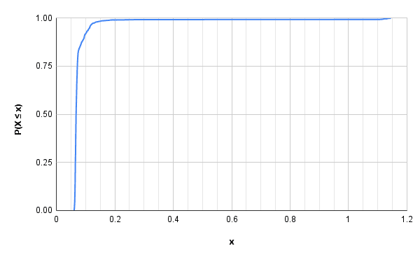
From the chart above you can say that most of the time (~99.9%), your service is under 0.2 ms. Fast!
The axis of the graph can be inverted to get a more "natural" look and highlight the increase in the "tail" latency. You can quickly look at this chart and "query" at which probability my service has which latency.
I personally love this.

Some measurements of above charts:
| P(X ≤ x) | x |
|---|---|
| 0.5 | 0.067 |
| 0.75 | 0.072 |
| 0.99 | 0.23 |
| 0.9995 | 1.12 |
| 0.9999 | 1.14 |
Table 8 My Service tail latency
Summary
Service latency should be communicated using probability.
An upper bound in service latency is a measure of service responsiveness and reliability. It is a guarantee that a service will always have latency under that value 100% of the time.
A more "relaxed" form of upper bound is called tail latency and it's a more practical way to explain service latency.
Describing latency using probability allows us to do some modeling & calculation that helps us make better engineering decisions. This might help save money.
Simple tools can be used to obtain an estimate of service latency probability from a sample measurement. You need to be mindful of how you take the sample and take the sample large enough to be representative.
Recommended Reads
[1] Applied Statistics and Probability for Engineers, 6th Edition. By By Douglas C. Montgomery, George C. Runger
[2] WHAT IS LATENCY AND HOW MUCH IS IT COSTING YOU by Eric Arrington.
[3] How Page Load Time Affects Bounce Rate and Page Views by Section.io
[4] ADDING AND SUBTRACTING PERCENTILES - HOW BAD CAN IT BE?(1995) by John G. Kreifeldt, Keoun Nah